
| 일 | 월 | 화 | 수 | 목 | 금 | 토 |
|---|---|---|---|---|---|---|
| 1 | ||||||
| 2 | 3 | 4 | 5 | 6 | 7 | 8 |
| 9 | 10 | 11 | 12 | 13 | 14 | 15 |
| 16 | 17 | 18 | 19 | 20 | 21 | 22 |
| 23 | 24 | 25 | 26 | 27 | 28 | 29 |
| 30 |
- docker
- Deeplearning
- COLAB
- Analog Rebellion
- CS
- 인디음악
- contiguous
- gru
- dl
- 자료구조
- pytorch
- vs code
- Algorithm
- torchtext
- 도커
- deep learning
- Transformation
- NLP
- tutorial
- Python
- rnn
- Data Structure
- lstm
- attention
- Today
- Total
Deep learning/Machine Learning/CS 공부기록
TEXT CLASSIFICATION WITH TORCHTEXT 본문
Introduction
이번 튜토리얼은 torchtext 내에 있는 text classification datasets을 어떻게 사용할 수 있는지 보여주고, 다음을 포함합니다.
- AG_NEWS,
- SogouNews,
- DBpedia,
- YelpReviewPolarity,
- YelpReviewFull,
- YahooAnswers,
- AmazonReviewPolarity,
- AmazonReviewFull
이 예제는 이러한 TextClassification datasets 중 하나를 이용하여 지도학습 분류 알고리즘을 어떻게 학습시키는지 보여줍니다.
본 튜토리얼은 파이토치 홈페이지 내의 튜토리얼을 번역한 자료입니다. 다수 의역이 되어있습니다. 역자주의 경우 지금과 같이 citation을 통해 남기도록 하겠습니다. 원문은 다음과 같습니다. 또한, 본 코드는 colab을 통해 실행할 수 있습니다. https://github.com/InhyeokYoo/PyTorch-tutorial-text/blob/master/TEXT_CLASSIFICATION_WITH_TORCHTEXT.ipynb
Load data with ngrams
A bag of ngrams features는 국소적인(local) 단어 순서에 대한 특정한 정보를 사로잡기 위해 이용됩니다. 실전에선 bi-gram이나 tri-gram은 단어의 그룹으로서 제공되어 단순히 하나의 단어만 이용하는 것보다 더 유용한 정보를 제공해줍니다.
"load data with ngrams"
Bi-grams results: "load data", "data with", "with ngrams"
Tri-grams results: "load data with", "data with ngrams"
TextClassification Dataset은 ngrams 메소드를 지원합니다. ngrams를 2로 세팅함으로써 dataset에 있는 예제 텍스트는 single words에 bi-grams string을 더한 list가 될 것입니다.
import torch
import torchtext
from torchtext.datasets import text_classification
# from torchtext.datasets import AG_NEWS # 다른 방법으로 importing하기
import os

NGRAMS = 2 # final로 선언합니다.

if not os.path.isdir('./.data'):
    os.mkdir('./.data')
train_dataset, test_dataset = text_classification.DATASETS['AG_NEWS'](
    root='./.data', ngrams=NGRAMS, vocab=None
)
BATCH_SIZE = 16
device = torch.device('cpu' if torch.cuda.is_available() == False else 'cuda')
print(device)
Define the model
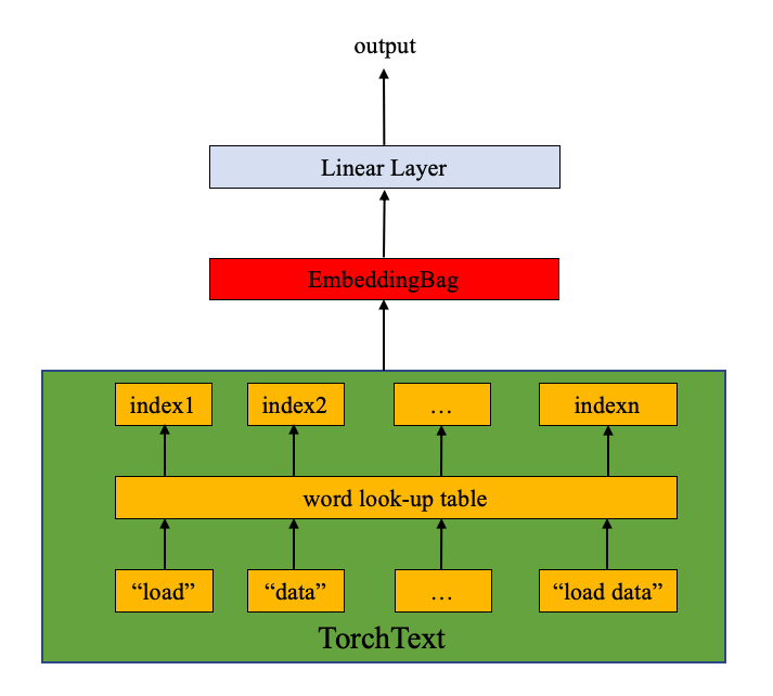
이 모델은 EmbeddingBag 레이어와 linear layer(밑에 그림 참고)로 이루어져 있습니다. nn.EmbeddingBag은 embedding 주머니(bag)의 평균값을 계산합니다. 튜토리얼의 text entries는 서로 다른 길이를 갖고 있습니다. nn.EmbeddingBag은 여기서 padding이 필요 없는데, 이는 offsets안에 텍스트의 길이가 저장되어 있기 때문입니다.
추가적으로, nn.EmbeddingBag은 평균을 즉석에서 누적하므로, nn.EmbeddingBag은 tensor의 시퀀스를 다룰 때 메모리 효율과 성능을 향상시킬 수 있습니다.
nn.EmbeddingBag은nn.Embedding후torch.mean(dim=0)와 동일합니다. 그러나,EmbeddingBag은 시간과 메모리면에서 훨씬 효율적입니다.
Input은Input(LongTensor),offsets(LongTensor, optional)으로,
- 만일
input이 (B, N)으로 2D이면, 각 길이가 고정으로N인B개의 주머니 (sequence)로 취급합니다. 이는mode에 따라 합산된B개의 값을 반환할 것이며,offsets는 이 경우에 무시됩니다. - 만일
input이 (N)의 1D라면, 여러 주머니(sequences)의 concatenation으로 취급합니다.offsets는 1D tensor로,input안의 각 주머니가 시작하는 지점의 index를 포함합니다. 따라서, (B) 차원의offsets에 대해서,input은B개의 주머니를 갖는다고 할 수 있습니다. 빈 주머니(즉, 0짜리 길이)는 0으로 채워진 tensor를 반환합니다.
import torch.nn as nn
import torch.nn.functional as F

class TextSentiment(nn.Module):
    def __init__(self, vocab_size: int, embed_dim: int, num_class: int):
        super(TextSentiment, self).__init__()
        self.embedding = nn.EmbeddingBag(num_embeddings=vocab_size, embedding_dim=embed_dim, sparse=True)
        self.fc = nn.Linear(embed_dim, num_class)
        self.init_weights()

    def init_weights(self):
        initrange = 0.5
        self.embedding.weight.data.uniform_(-initrange, initrange)
        self.fc.weight.data.uniform_(-initrange, initrange)
        self.fc.bias.data.zero_()

    def forward(self, text, offsets):
        embedded = self.embedding(text, offsets)
        return self.fc(embedded)
Initiate an instance
AG_NEWS 데이터셋은 네 개의 레이블이있고, 따라서 클래스의 갯수는 4가 됩니다.
1 : World
2 : Sports
3 : Business
4 : Sci/Tec
사전의 크기(vocab size)는 사전(vocab; 개별 단어와 ngrams를 포함)의 길이와 같습니다. 클래스의 개수는 레이블의 개수와 같고, AG_NEWS의 경우 4가 됩니다.
VOCAB_SIZE = len(train_dataset.get_vocab())
EMBED_DIM = 32
NUN_CLASS = len(train_dataset.get_labels())
model = TextSentiment(VOCAB_SIZE, EMBED_DIM, NUN_CLASS).to(device)
VOCAB_SIZE = len(train_dataset.get_vocab())
EMBED_DIM = 32
NUN_CLASS = len(train_dataset.get_labels())
model = TextSentiment(VOCAB_SIZE, EMBED_DIM, NUN_CLASS).to(device)Functions used to generate batch
다음 요소가 서로 다른 길이를 갖기때문에, 사용자 함수인 generate_batch()를 이용하여 data batches와 offsets를 생성합니다. 이 함수는 torch.utils.data.DataLoader안에 있는 collate_fn으로 전달됩니다. collate_fn의 인풋은 batch_size만큼의 크기를 갖는 tensors로 이루어진 list이고, collate_fn 함수는 mini_batch로 나눕니다. collate_fn은 최고 레벨의 함수로 선언되는 것에 주목합시다. 이는 이 함수가 각 worker에서 사용가능하게 합니다.
원본 data batch input의 텍스트는 list로 감싸져있고, 하나의 tensor로 concat되어 nn.EmbeddingBag의 input이 됩니다. Offset은 text tensor내 개별 sequence의 시작점의 인덱스를 나타내는 텐서입니다.
torchtext.datasets.TextClassificationDataset의 data에 대한 설명은 다음과 같습니다: label/tokens의 튜플로 이루어진 리스트로, tokens은 string tokens를 numericalizing한 것이고, label은 integer입니다.[(label1, tokens1), (label2, tokens2), (label2, tokens3)]
def generate_batch(batch):
    label = torch.tensor([entry[0] for entry in batch])
    text = [entry[1] for entry in batch]
    offsets = [0] + [len(entry) for entry in text]
    # torch.tensor.cumsum은 정해진 dimension dim
    # 안에 요소의 누적합을 반환합니다.
    # torch.Tensor([1.0, 2.0, 3.0]).cumsum(dim=0)

    offsets = torch.tensor(offsets[:-1]).cumsum(dim=0)
    text = torch.cat(text)
    return text, offsets, label
Define functions to train the model and evaluate results.
torch.utils.data.DataLoader는 손쉽게 병렬 데이터 로딩을 가능케하고 PyTorch 사용자에게 권장됩니다. 여기서는 DataLoader를 사용하여 AG_NEWS 데이터셋을 불러오고 모델로 보내 training과 validation을 해보도록 하겠습니다.
from torch.utils.data import DataLoader

def train_func(sub_train_):
    # Train the model
    train_loss = 0
    train_acc = 0

    data = DataLoader(sub_train_, batch_size=BATCH_SIZE, shuffle=True, collate_fn=generate_batch)
    for i, (text, offsets, cls) in enumerate(data):
        optimizer.zero_grad()
        text, offsets, cls = text.to(device), offsets.to(device), cls.to(device)
        output = model(text, offsets)
        loss = criterion(output, cls)
        train_loss += loss.item()
        loss.backward()
        optimizer.step()
        # 마지막엔 softmax layer를 추가해도 좋습니다.
        train_acc += (output.argmax(1) == cls).sum().item()

    # Learning rate 조정
    scheduler.step()

    return train_loss / len(sub_train_), train_acc / len(sub_train_)

def test(data_):
    loss = 0
    acc = 0
    data = DataLoader(data_, batch_size=BATCH_SIZE, collate_fn=generate_batch)

    for text, offsets, cls in data:
        text, offsets, cls = text.to(device), offsets.to(device), cls.to(device)
        with torch.no_grad():
            output = model(text, offsets)
            loss = criterion(output, cls)
            loss += loss.item()
            # 마지막엔 softmax layer를 추가해도 좋습니다.
            acc += (output.argmax(1) == cls).sum().item()

    return loss / len(data_), acc / len(data_)
살짝 헷갈리므로 불러오는 데이터의 형식을 한번 살펴보도록 하겠습니다. Tractable 하기위해
shuffle=False로 설정하겠습니다.
data = DataLoader(train_dataset, batch_size=BATCH_SIZE, shuffle=False, collate_fn=generate_batch)
for i, (text, offsets, cls) in enumerate(data):
    print(f"text: {text}, len: {len(text)}")
    print(f"offsets: {offsets}, length:{len(offsets)}")
    print(f"cls: {cls}, len: {len(cls)}")
    print("="*200)
    if i == 3:
        break
text: tensor([ 572, 564, 2, ..., 1194110, 300136, 10278]), len: 1432
offsets: tensor([ 0, 57, 140, 219, 298, 383, 478, 571, 668, 843, 904, 991,
1102, 1163, 1262, 1369]), length:16
cls: tensor([2, 2, 2, 2, 2, 2, 2, 2, 2, 2, 2, 2, 2, 2, 2, 2]), len: 16
========================================================================================================================================================================================================
text: tensor([ 6312, 1934, 12, 11087, 3, 22219, 518, 7,
6312, 24, 6, 330, 483, 7, 1616, 3,
11087, 160, 33, 805, 749, 6, 1662, 2240,
32572, 2, 902849, 75962, 98359, 607543, 285041, 1066517,
15746, 75193, 902829, 748, 2338, 86787, 711, 90638,
13928, 92801, 58329, 43326, 3790, 326457, 9257, 3783,
854300, 941058, 133813, 8, 6, 185, 172, 4,
491, 1150, 2629, 1675, 311, 24, 729, 2347,
12, 8779, 8, 3, 397, 172, 1772, 406,
4, 55, 484, 8, 1264126, 3234, 1675, 49,
3409, 5, 4556, 6, 3972, 205647, 67, 213,
389, 409, 90, 17, 2199, 807, 961, 95,
3, 12710, 99, 10167, 20, 339, 2, 69,
95020, 736002, 2851, 17829, 374787, 1237903, 1264092, 805618,
2747, 68653, 257462, 34483, 186016, 108979, 26, 5641,
4893, 398378, 9078, 4636, 118, 58487, 21111, 865376,
1264127, 8199, 128097, 74027, 9735, 30707, 110726, 5686,
628300, 1153763, 20034, 49689, 90771, 8704, 4062, 5581,
93577, 929207, 1867, 3013, 50849, 110950, 1287945, 164313,
213522, 6660, 45, 365, 1742, 83790, 8, 2850,
3, 45, 365, 1742, 33, 2741, 1202, 5,
6, 198, 6510, 2, 30845, 21, 78, 708,
4155, 4997, 379, 4, 287, 5, 6, 415,
2134, 2, 12477, 6830, 109897, 1189362, 8652, 388782,
243, 12477, 6830, 237651, 55629, 765573, 71724, 120,
1846, 91472, 34265, 36919, 534938, 2339, 34997, 125739,
739261, 861166, 10875, 356, 292, 120, 220766, 100118,
24234, 4793, 17, 125, 47, 1045, 12, 1852,
17, 78, 334, 4793, 125, 47, 25346, 2290,
12, 6, 938, 1374, 4, 4239, 34, 573,
622, 1852, 4, 6, 445, 201, 763, 2,
205030, 77575, 893, 325961, 12783, 88414, 1236518, 169373,
4176, 59244, 443323, 893, 325695, 230304, 47142, 159,
10752, 60980, 62410, 14159, 1049256, 88523, 245327, 1101491,
210559, 87, 11236, 60403, 432179, 29108, 271, 2394,
1278, 16001, 117357, 3, 7356, 714, 9982, 12,
271, 17, 10, 513, 978, 4, 467, 10354,
1764, 48, 35, 2657, 20, 25, 16676, 8,
16001, 3161, 2, 17671, 880443, 768722, 1042460, 1151655,
29673, 625374, 59242, 84515, 26125, 9219, 23, 31602,
3878, 16807, 2405, 723052, 910659, 15083, 11985, 6514,
12892, 1769, 386528, 96424, 251636, 101870, 11022, 10331,
469, 2864, 1097, 396, 2134, 684, 3, 94648,
10331, 469, 1668, 5, 3091, 4, 55, 311,
52, 4479, 30, 137, 1785, 185, 1508, 8,
3, 94, 2, 80023, 745580, 192332, 825782, 22182,
31177, 16039, 103962, 218068, 80023, 110300, 3850, 6498,
59288, 118, 6605, 3430, 320282, 291116, 3810, 32452,
27156, 735987, 12904, 26, 1011, 682, 2509, 8597,
8, 259, 489, 339, 8, 259, 8597, 185,
21, 3, 244, 24219, 6, 902, 8, 2418,
9, 1035, 1082, 2, 764286, 56910, 2320, 891739,
2262, 2410, 2320, 891913, 92233, 7696, 194, 428,
700072, 184707, 7882, 2372, 63662, 46665, 16655, 87467,
15504, 28692, 1661, 11, 3575, 5737, 873, 374,
782, 818, 52, 22854, 5, 412, 2, 336,
28, 3, 289, 1059, 745, 255, 4, 55,
3, 3605, 7, 1282, 840, 3, 28692, 9,
17783, 975, 2, 1076001, 18610, 1006034, 1141777, 1114946,
429101, 708148, 1683, 64842, 590747, 288299, 14131, 2836,
854, 219269, 207, 3689, 4348, 557636, 3740, 4170,
118, 837, 19174, 4251, 264657, 474106, 22593, 137995,
1075998, 317874, 1187133, 5961, 493, 124, 185, 799,
3, 678, 3, 1064, 7, 1879, 643, 27,
9, 173, 1649, 2531, 582, 1896, 48, 3,
476, 335, 130, 4, 6, 27, 1206, 33,
443, 2, 147011, 60410, 352073, 1630, 4311, 46421,
5839, 4281, 47430, 649660, 146232, 16528, 32011, 1128045,
830772, 660740, 15668, 277998, 204, 1286, 45200, 3633,
1255, 87, 151, 21172, 83783, 6615, 12878, 289,
557, 8963, 782, 818, 289, 557, 17, 10,
745, 255, 738, 782, 818, 28, 6, 353,
9845, 1310, 5, 297, 2, 336, 8, 6,
307, 5, 1190, 339, 8, 3, 469, 2,
2148, 905803, 930413, 1683, 1077451, 2148, 8051, 23,
10711, 3740, 227697, 708442, 1683, 27084, 514, 8765,
82786, 27053, 11989, 17216, 2251, 854, 26601, 69,
2630, 1324, 8524, 149492, 2410, 26, 1877, 4261,
271, 2325, 2081, 11, 86, 35, 2325, 7,
249, 8, 271, 4, 3, 305, 238, 985,
136, 125, 47, 23622, 12, 21, 519, 21,
307773, 4, 720, 780, 11, 86, 2, 819593,
602813, 51767, 193, 111243, 20497, 16668, 16534, 4002,
28481, 9596, 42, 2628, 5551, 1269, 355827, 6262,
893, 615034, 786442, 24240, 2639, 3163, 593794, 538085,
25882, 48015, 15000, 193, 558, 1494, 249, 10616,
11, 209, 186, 2771, 249, 566, 40, 3622,
785, 883, 4, 304, 3, 436, 1522, 3,
295, 353, 39, 604, 566, 1292, 7, 1357,
2, 853804, 60759, 84464, 30434, 425407, 407335, 249303,
11179, 34645, 48710, 87754, 15807, 12436, 1027, 2878,
5128, 243396, 84693, 1012, 150771, 102202, 16093, 314939,
24227, 4861, 39375, 6612, 944226, 9335, 436, 738,
447, 82, 7, 3, 10701, 9335, 5251, 11,
3, 948, 5250, 1382, 7, 399086, 92, 113,
3023, 623, 6152, 9, 374, 10187, 447, 2,
944227, 1203085, 782156, 62895, 894646, 283, 29, 20845,
1003097, 1203094, 1011019, 79, 6102, 47059, 263709, 9048,
995233, 944228, 605, 475382, 444192, 1137012, 52209, 14611,
73146, 25909, 10684, 6180, 1369, 3755, 886, 34,
5465, 6180, 3587, 3, 5465, 12, 6, 5923,
5, 477, 12, 1112, 40, 56, 95, 1009,
4, 219, 5474, 34, 181073, 614, 8, 1115,
722, 2, 665893, 277044, 1085426, 58078, 366974, 860022,
665870, 51665, 41643, 379955, 159, 106665, 37664, 1197,
7534, 244361, 257785, 14174, 192, 6215, 10100, 223,
106117, 82914, 801917, 690986, 55184, 6531, 20894, 25114,
259, 378, 436, 12450, 4612, 3, 72, 802,
3, 647, 378, 1821, 313, 28, 6, 10120,
5153, 24, 5, 551, 25, 53338, 12, 1456,
6466, 2, 387544, 989428, 362050, 1144616, 1041916, 202,
686927, 16025, 3967, 130283, 56299, 1041765, 3822, 514,
43934, 242516, 550834, 1451, 4543, 26753, 386890, 1079358,
80327, 116774, 96841, 3043, 18284, 8, 172, 12708,
43629, 614261, 4, 3, 3043, 18284, 5393, 12,
4104, 3, 799810, 339840, 939, 4, 24, 2129,
5, 12708, 38, 72, 11, 3, 397, 172,
2, 472271, 878834, 25512, 940622, 786434, 1242042, 614262,
42, 20849, 472271, 878830, 59022, 59117, 18963, 1209783,
799811, 678659, 30520, 734, 7373, 4830, 57284, 786418,
9712, 29117, 79, 5641, 4893, 1818]), len: 966
offsets: tensor([ 0, 51, 154, 217, 278, 335, 390, 433, 500, 559, 624, 685, 740, 795,
856, 907]), length:16
cls: tensor([2, 2, 2, 2, 2, 2, 2, 2, 2, 2, 2, 2, 2, 2, 2, 2]), len: 16
========================================================================================================================================================================================================
text: tensor([ 2226, 4547, 5, ..., 1083638, 24519, 11559]), len: 1552
offsets: tensor([ 0, 71, 138, 189, 252, 353, 450, 587, 738, 907, 1010, 1077,
1196, 1321, 1402, 1467]), length:16
cls: tensor([2, 2, 2, 2, 2, 2, 2, 2, 2, 2, 2, 2, 2, 2, 2, 2]), len: 16
========================================================================================================================================================================================================
text: tensor([ 12, 1001, 3, ..., 53174, 37, 37]), len: 1296
offsets: tensor([ 0, 75, 110, 151, 208, 271, 354, 403, 440, 479, 522, 641,
818, 911, 1078, 1187]), length:16
cls: tensor([2, 2, 2, 2, 2, 2, 2, 2, 2, 2, 2, 2, 2, 2, 2, 2]), len: 16이로 미루어 알 수 있는 사실은 16개 (
len(offsets)orlen(cls))의 sequences (bags)가 text 안에 담겨있고, offsets는 각 bag의 시작점을 알려주고 있습니다. 각 bag의 길이는 모두 서로 다릅니다. 본 데이터 셋은 [Batch x length]를 반환하는 대신, [BATCH_SIZE] concat된 bag과 offsets를 반환합니다.
참고로 원래의 dataset은 다음과 같이 생겼습니다.
data = DataLoader(train_dataset, shuffle=False)
for i, (x) in enumerate(data):
    print(x, x[1].size())
    print("="*200)
    if i == 3:
        break
# Result
[tensor([2]), tensor([[ 572, 564, 2, 2326, 49106, 150, 88, 3,
1143, 14, 32, 15, 32, 16, 443749, 4,
572, 499, 17, 10, 741769, 7, 468770, 4,
52, 7019, 1050, 442, 2, 14341, 673, 141447,
326092, 55044, 7887, 411, 9870, 628642, 43, 44,
144, 145, 299709, 443750, 51274, 703, 14312, 23,
1111134, 741770, 411508, 468771, 3779, 86384, 135944, 371666,
4052]])] torch.Size([1, 57])모든 데이터를 다 확인할 순 없지만 앞서
collate_fn을 이용한 결과와 위의 결과를 비교하면BATCH_SIZE만큼 데이터를 concat하여 사용함을 확인할 수 있습니다.
Split the dataset and run the model
원본 AG_NEWS 데이터에는 validation set이 없으므로 training set을 0.95의 비율로 나누겠습니다. 이를 위해 우리는 torch.utils.data.datasets.random_split을 사용하겠습니다.
CrossEntropyLoss는 nn.LogSoftmax()와 nn.NLLLoss()를 하나로 합쳐놓은 것입니다. 이는 C개의 클래스를 분류하는 문제를 학습시킬 때 유용합니다. SGD는 stochastic gradient descent를 optimizer로서 구현한 것입니다. 초기 learning rate값은 4.0으로 설정되어있습니다. StepLR은 여기서 epochs에 따라 learning rate를 조절하기 위해 사용되었습니다.
import time
from torch.utils.data.dataset import random_split

N_EPOCHS = 5
min_valid_loss = float('inf')   # 왜 있는지 모르겠음

criterion = torch.nn.CrossEntropyLoss().to(device)
optimizer = torch.optim.SGD(model.parameters(), lr=4.0)
# StepLR은 step_size마다 lr을 gamma만큼 줄여서 작동한다: 이 경우, 4.0, 3.6, ..., 로 줄어든다.
scheduler = torch.optim.lr_scheduler.StepLR(optimizer=optimizer, step_size=1, gamma=0.9)

train_len = int(len(train_dataset) * 0.95)
# random_split(dataset: Dataset, lengths: 'sequence')
# Arguments:
#        dataset (Dataset): Dataset to be split
#        lengths (sequence): lengths of splits to be produced
sub_train_, sub_valid_ = random_split(dataset=train_dataset, lengths=[train_len, len(train_dataset) - train_len])

for epoch in range(N_EPOCHS):
    start_time = time.time()
    train_loss, train_acc = train_func(sub_train_)
    valid_loss, valid_acc = test(sub_valid_)

    secs = int(time.time() - start_time)
    mins = secs / 60
    secs = secs % 60

    # f string
    print(f'Epoch: {epoch + 1}', f" | time in {mins} minutes, {secs} seconds")
    print(f'\tLoss: {train_loss:.4f}(train)\t|\tAcc: {train_acc * 100:.1f}%(train)')
    print(f'\tLoss: {valid_loss:.4f}(valid)\t|\tAcc: {valid_acc * 100:.1f}%(valid)')
Epoch: 1 | time in 0.13333333333333333 minutes, 8 seconds
Loss: 0.0126(train) | Acc: 93.3%(train)
Loss: 0.0001(valid) | Acc: 93.2%(valid)
Epoch: 2 | time in 0.13333333333333333 minutes, 8 seconds
Loss: 0.0071(train) | Acc: 96.2%(train)
Loss: 0.0001(valid) | Acc: 93.1%(valid)
Epoch: 3 | time in 0.13333333333333333 minutes, 8 seconds
Loss: 0.0039(train) | Acc: 98.1%(train)
Loss: 0.0000(valid) | Acc: 93.0%(valid)
Epoch: 4 | time in 0.13333333333333333 minutes, 8 seconds
Loss: 0.0023(train) | Acc: 98.9%(train)
Loss: 0.0001(valid) | Acc: 93.4%(valid)
Epoch: 5 | time in 0.13333333333333333 minutes, 8 seconds
Loss: 0.0014(train) | Acc: 99.4%(train)
Loss: 0.0000(valid) | Acc: 93.8%(valid) Evaluate the model with test dataset
print('Checking the results of test dataset...')
test_loss, test_acc = test(test_dataset)
print(f'\tLoss: {test_loss:.4f}(test)\t|\tAcc: {test_acc * 100:.1f}%(test)')
Test on a random news
제일 좋은 모델을 사용하여 골프 뉴스를 테스트해보자. label정보는 이곳에서 확인할 수 있다.
from torchtext.data.utils import ngrams_iterator
from torchtext.data.utils import get_tokenizer

ag_news_label = {1 : "World",
                 2 : "Sports",
                 3 : "Business",
                 4 : "Sci/Tec"}

def predict(text, model, vocab, ngrams):
    tokenizer = get_tokenizer("basic_english")
    with torch.no_grad():
        text = torch.tensor([vocab[token]
                            for token in ngrams_iterator(tokenizer(text), ngrams)])
        output = model(text, torch.tensor([0]))
        return output.argmax(1).item() + 1

ex_text_str = "MEMPHIS, Tenn. – Four days ago, Jon Rahm was \
    enduring the season’s worst weather conditions on Sunday at The \
    Open on his way to a closing 75 at Royal Portrush, which \
    considering the wind and the rain was a respectable showing. \
    Thursday’s first round at the WGC-FedEx St. Jude Invitational \
    was another story. With temperatures in the mid-80s and hardly any \
    wind, the Spaniard was 13 strokes better in a flawless round. \
    Thanks to his best putting performance on the PGA Tour, Rahm \
    finished with an 8-under 62 for a three-stroke lead, which \
    was even more impressive considering he’d never played the \
    front nine at TPC Southwind."

vocab = train_dataset.get_vocab()
model = model.to("cpu")

print("This is a %s news" %ag_news_label[predict(ex_text_str, model, vocab, 2)])'ML, DL > NLP' 카테고리의 다른 글
| SEQUENCE-TO-SEQUENCE MODELING WITH NN.TRANSFORMER AND TORCHTEXT (0) | 2020.06.29 |
|---|---|
| LANGUAGE TRANSLATION WITH TORCHTEXT (0) | 2020.06.29 |
| PyTorch Attention 구현 issue 정리 (0) | 2020.06.18 |
